
Time series forecasting has long been the backbone of critical business decisions, where data scientists relied on classical statistical methods like ARIMA, Exponential Smoothing, and their seasonal variants. These approaches, while interpretable and well-understood, require significant domain expertise, manual parameter tuning, and often struggle with the complex, non-linear patterns present in real-world data.
The rise of deep learning brought new possibilities, but also new challenges. Models like LSTMs and early Transformer variants showed promise but demanded large amounts of training data and extensive hyperparameter optimization for each new forecasting task. The question remained: could we build a single model that generalizes across diverse time series domains, much like GPT revolutionized natural language processing?
In this blog post, we’ll explore:
- How Transformer architectures have been adapted for time series forecasting
- The innovative design behind Chronos-2
- A comprehensive evaluation comparing Chronos-2 against classical baselines
- Detailed analysis across four diverse benchmark datasets
In this post I’ll try to compare transformer models with statistical models, which in my opinion is not an apples-to-apples comparison. However, to be fair, there’s no data massaging, feature extraction, or hyperparameter tuning (except for ARIMA: Auto ARIMA is a common baseline). The idea here is to mimic day 0 at an AI/Data Lab: take the dataset and run your model pipeline evals to create baselines.
Transformers for Time Series
The Transformer architecture, introduced in “Attention Is All You Need” paper, revolutionized natural language processing with its self-attention mechanism. Unlike recurrent neural networks (RNNs) that process sequences step-by-step, Transformers can attend to all positions in a sequence simultaneously, capturing long-range dependencies more effectively.
The key insight that made Transformers applicable to time series was recognizing that forecasting is fundamentally a sequence-to-sequence problem. Just as language models predict the next word given context, time series models predict future values given historical observations.
Self-Attention Mechanism
The self-attention mechanism enables the model to weigh the importance of different time steps when making predictions. For time series, this matters a lot. Example: Yesterday’s sales often predict today’s, which captures those short-term patterns we rely on. But we also need to look further back, seasonal patterns from a year ago can inform current forecasts just as much. And then there are those irregular events, like holiday effects or anomalies from months past, that might still be influencing what’s happening now.
Positional Encoding
Since Transformers are inherently order-agnostic, positional information must be explicitly encoded. For time series, this goes beyond simple positional indices. We’re talking about temporal embeddings that capture the hour of day, day of week, or month of year. There’s also the concept of relative positions, which tells the model how far apart two time steps actually are. And of course, calendar features like holidays, weekends, and special events add another layer of context that helps the model understand what’s really going on in the data.
Chronos-2: Universal Time Series Forecasting
Developed by Amazon, Chronos-2 is a 120M-parameter encoder-only model that can tackle univariate, multivariate, and covariate-informed forecasting tasks without any task-specific training. It draws inspiration from the T5 encoder architecture and produces probabilistic forecasts across 21 quantile levels, giving you a detailed picture of prediction uncertainty.
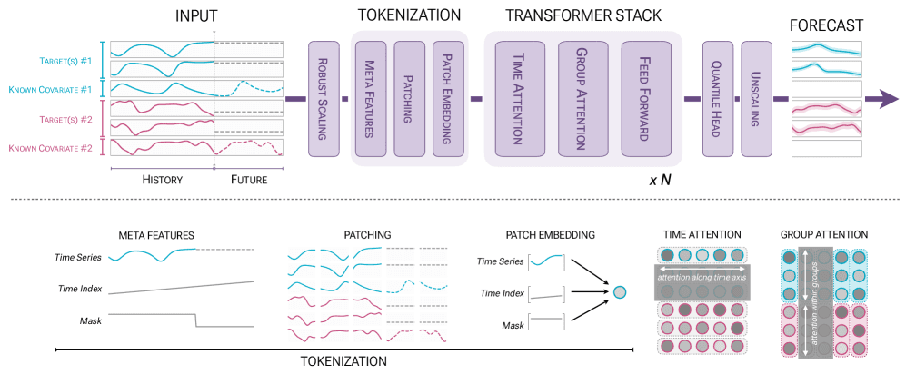
Group Attention
The architectural breakthrough behind Chronos-2 is its group attention mechanism, which enables true in-context learning across multiple related time series. Instead of processing each series in isolation, the model alternates between two types of attention layers. Time attention operates along the temporal axis within each individual series, using standard self-attention with rotary position embeddings (RoPE). Group attention then operates across all series within a group at each time step, allowing the model to share information between variates.
What makes this elegant is how the group attention layer handles information sharing. Rather than extending the context window by concatenating all targets and covariates together (which scales poorly), it shares information across the batch dimension within defined groups. This lets the model scale gracefully as you add more variates. When forecasting cloud metrics, for instance, patterns in CPU usage can directly inform memory consumption predictions. The same mechanism naturally handles covariates, incorporating information from promotional schedules or weather forecasts into demand predictions.
Groups themselves are flexible. They can represent arbitrary collections of related univariate series, the different variates of a multivariate system, or targets paired with their associated covariates. Importantly, the group attention layer omits positional encoding since the order of series within a group shouldn’t affect the output.
Synthetic Data Training
Building a universal forecasting model requires training data that covers diverse multivariate relationships and informative covariate structures. The problem is that high-quality real-world data with these properties is remarkably scarce. Chronos-2 addresses this through a clever synthetic data generation strategy.
The key innovation is what the team calls “multivariatizers.” These take time series from base univariate generators (including autoregressive models, exponential smoothing, and KernelSynth) and impose dependencies among them to create realistic multivariate dynamics. Some multivariatizers create aligned relationships where series move together, while others introduce lagged dependencies that simulate real-world causal structures. The team also employed generators like TSI (which combines trend, seasonality, and irregularity components) and TCM (which samples from random temporal causal graphs).
For multivariate and covariate-informed forecasting specifically, Chronos-2 relies entirely on synthetic data. The results validate this approach: ablation studies show that models trained only on synthetic data perform nearly as well as those trained on a mixture of real and synthetic datasets. This suggests that carefully designed synthetic generation may be sufficient for pretraining time series models, opening the door to even more capable future models without requiring massive real-world data collection efforts.
Chronos-2 achieves state-of-the-art zero-shot performance across three major benchmarks (fev-bench, GIFT-Eval, and Chronos Benchmark II), with especially large gains on tasks involving covariates. Against its predecessor Chronos-Bolt, it achieves a win rate exceeding 90% in head-to-head comparisons.
Datasets and Evaluations
In our experiments, we evaluated four configurations of Chronos-2 and three statistical methods:
- chronos2: Zero-shot prediction using the pretrained model directly
- chronos2-cov: Zero-shot with covariates (time features + dataset-specific variables)
- chronos2-ft: Full fine-tuning on the target dataset
- chronos2-ft-lora: Parameter-efficient fine-tuning using LoRA (Low-Rank Adaptation)
- Arima: Sarimax from statsmodels
- Auto-Arima: Sarimax optimal parameter selection
- Holt-Winters: Exponential smoothing
We evaluated our models on four diverse datasets, each presenting its own forecasting challenges: Air Passengers, ETTh1, Traffic and Weather.
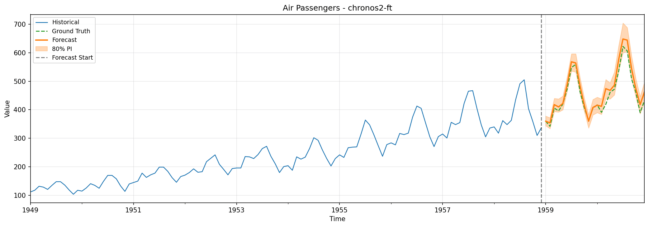
Air Passengers
This classic dataset records monthly totals of international airline passengers (in thousands) from January 1949 through December 1960 (just 144 observations of a single time series). Despite its simplicity, Air Passengers remains a gold standard in time series analysis because it contains textbook examples of the patterns any forecasting model must handle: a clear upward trend as air travel grew more popular, strong annual seasonality with summer peaks, and crucially, the interaction between the two where seasonal swings grow larger as the overall numbers climb.
We held out the final 24 months for testing.
| Model | MAE | RMSE | MAPE (%) | SMAPE (%) | MASE | Coverage (%) | Interval Width |
|---|---|---|---|---|---|---|---|
| chronos2 | 36.95 | 41.59 | 7.91 | 8.31 | 0.82 | 62.5 | 90.74 |
| chronos2-cov | 43.43 | 47.12 | 9.42 | 9.95 | 0.96 | 58.3 | 98.48 |
| chronos2-ft | 17.75 | 22.70 | 3.83 | 3.71 | 0.39 | 91.7 | 60.25 |
| chronos2-ft-lora | 25.25 | 29.99 | 5.48 | 5.28 | 0.56 | 50.0 | 49.67 |
| arima | 69.90 | 75.63 | 15.22 | 16.65 | 1.55 | 4.2 | 93.13 |
| auto-arima | 43.46 | 47.23 | 9.44 | 9.97 | 0.96 | 4.2 | 49.19 |
| holt-winters | 31.08 | 35.76 | 6.64 | 6.92 | 0.69 | 95.8 | 99.42 |
Fine-tuned Chronos-2 dominates here, achieving a MAE of 17.75 compared to the next best 25.25, with MAPE under 4%. Even without any training on this dataset, the zero-shot model hits a MASE of 0.82 (outperforming the naïve baseline by 18%).
A few surprises emerged. Adding covariates actually hurt performance slightly on this univariate dataset, suggesting the model may have been overfitting to time features that weren’t providing useful signal. Manual ARIMA configuration performed poorly with a MASE of 1.55, worse than simply predicting the last observed value. On the other hand, Holt-Winters elivered excellent coverage at 95.8% alongside competitive point forecasts.
For datasets with clear, established patterns like this one, fine-tuning delivers dramatic improvements. Both fine-tuned Chronos-2 and Holt-Winters successfully captured the multiplicative seasonality where amplitude grows with trend.
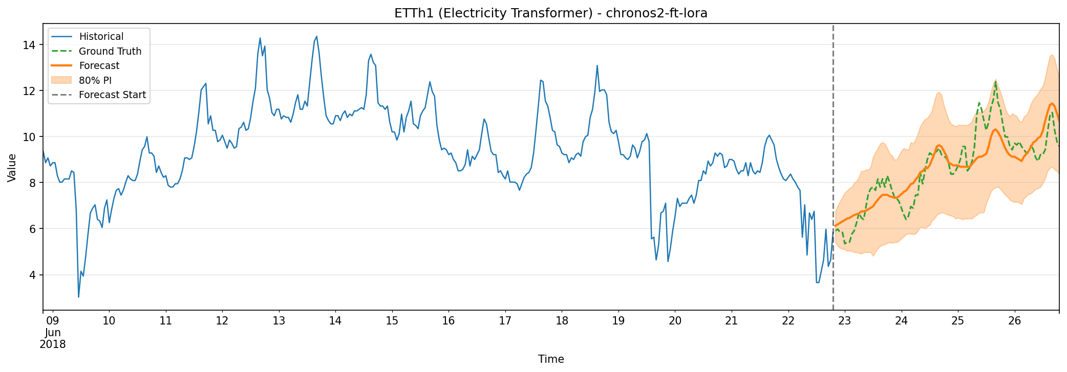
ETTh1 (Electricity Transformer Temperature)
Moving to something more complex, the ETTh1 dataset monitors an electricity transformer in China from July 2016 to July 2018. The target variable is oil temperature, recorded hourly alongside six load features representing different types of power consumption. With roughly 17,000 observations, this dataset presents multiple challenges: daily patterns nested within weekly cycles, irregular load variations that don’t follow simple cyclical behavior, and multivariate relationships where oil temperature depends on those load patterns.
This benchmark was introduced with the Informer paper and has become standard for long-sequence forecasting. Getting transformer temperature right helps prevent equipment failures and optimize power distribution. We tested on a 96-hour (4-day) forecast horizon.
| Model | MAE | RMSE | MAPE (%) | SMAPE (%) | MASE | Coverage (%) | Interval Width |
|---|---|---|---|---|---|---|---|
| chronos2 | 1.22 | 1.47 | 13.29 | 14.20 | 3.81 | 96.9 | 6.59 |
| chronos2-cov | 1.17 | 1.44 | 12.89 | 14.04 | 3.65 | 86.5 | 4.50 |
| chronos2-ft | 1.13 | 1.37 | 12.43 | 13.30 | 3.54 | 88.5 | 4.15 |
| chronos2-ft-lora | 0.65 | 0.81 | 7.51 | 7.50 | 2.02 | 97.9 | 3.98 |
| arima | 3.25 | 3.57 | 35.70 | 44.74 | 10.15 | 99.0 | 9.99 |
| auto-arima | 2.82 | 3.23 | 30.18 | 36.97 | 8.82 | 100.0 | 10.70 |
| holt-winters | 3.21 | 3.52 | 35.26 | 44.04 | 10.03 | 99.0 | 10.52 |
LoRA fine-tuning achieved remarkable results here, with a MAE of 0.65 (nearly half that of full fine-tuning). There’s a clear hierarchy visible in the results: zero-shot → covariates → fine-tuning → LoRA, suggesting the model effectively leverages each additional source of information.
Classical methods, meanwhile, failed dramatically. All statistical baselines have MASE above 8, meaning they’re 8x worse than the naïve forecast. The complex patterns in transformer temperature data simply defeat traditional approaches. LoRA also achieved the best uncertainty quantification: 97.9% coverage with the narrowest prediction intervals.
ETTh1 showcases the power of foundation models. The irregular patterns and multivariate dependencies here are beyond what classical methods can capture, but Chronos-2 handles them effectively.
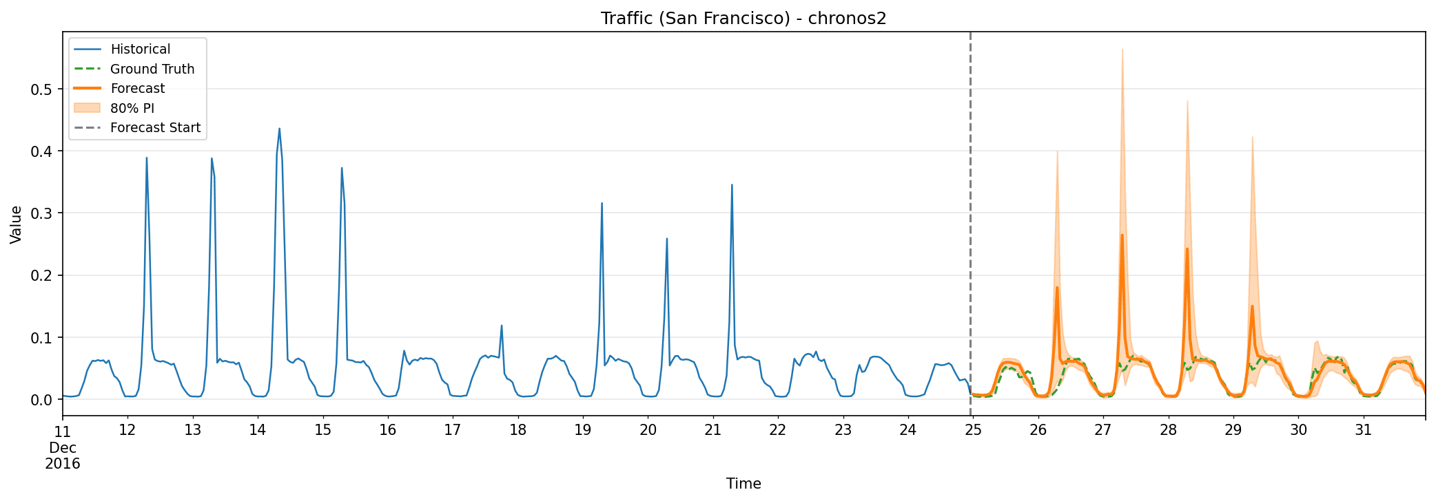
Traffic (California Freeway Occupancy)
This large-scale dataset from the California Department of Transportation contains road occupancy rates measured by 862 sensors across San Francisco Bay area freeways from January 2015 through December 2016. That’s roughly 15 million total observations. Traffic data presents unique difficulties: the sheer number of series requires scalable approaches, traffic at one location affects nearby sensors, and there are complex seasonal patterns including rush hour, weekend effects, and holiday variations. The occupancy values range from 0 to 1, with nighttime readings often near zero.
We tested 96-hour forecasts for each sensor.
| Model | MAE | RMSE | MAPE (%) | SMAPE (%) | MASE | Coverage (%) | Interval Width |
|---|---|---|---|---|---|---|---|
| chronos2 | 0.0132 | 0.0299 | 43.92 | 37.65 | 1.57 | 74.0 | 0.038 |
| chronos2-cov | 0.0134 | 0.0304 | 47.22 | 39.46 | 1.60 | 73.3 | 0.039 |
| chronos2-ft | 0.0142 | 0.0317 | 43.01 | 36.65 | 1.69 | 69.6 | 0.035 |
| chronos2-ft-lora | 0.0143 | 0.0316 | 43.84 | 37.50 | 1.70 | 66.6 | 0.034 |
| arima | 0.0278 | 0.0427 | 186.09 | 87.59 | 3.31 | 99.7 | 0.694 |
| auto-arima | 0.0284 | 0.0411 | 369.35 | 71.50 | 3.38 | 92.9 | 0.144 |
| holt-winters | 0.1087 | 0.2763 | 1078.24 | 100.90 | 12.95 | 86.0 | 0.617 |
Here’s something interesting: zero-shot Chronos-2 performed best on point metrics, and fine-tuning actually hurt performance. Both fine-tuning approaches slightly worsened results, possibly due to overfitting on the limited training window.
You’ll notice the MAPE exceeds 40% despite good MAE. This apparent paradox comes from the near-zero nighttime values, dividing by small numbers inflates percentage errors dramatically. Holt-Winters collapsed entirely with MAPE over 1000%, indicating catastrophic failure on this multi-series dataset.
The lesson from traffic data is important: more training isn’t always better. The zero-shot model’s general knowledge transfers well to traffic patterns, while fine-tuning may overfit to local patterns that don’t generalize across the 862 diverse sensors.
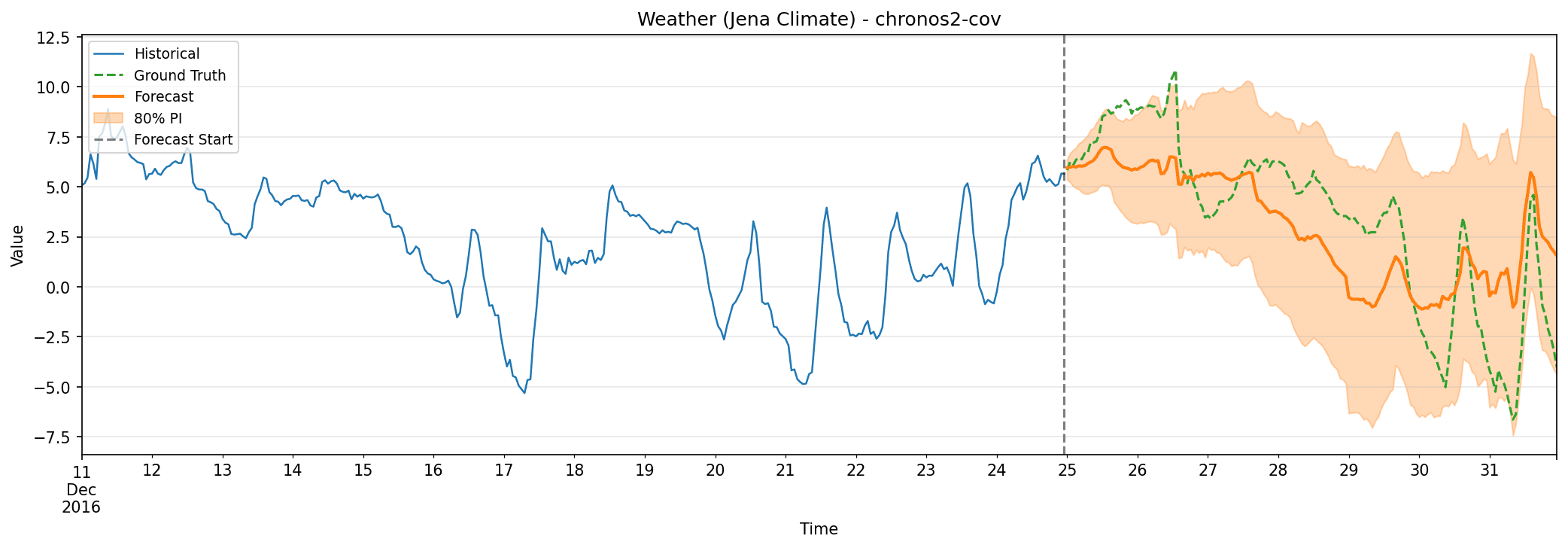
Weather (Jena Climate)
Our final dataset comes from the Max Planck Institute for Biogeochemistry in Germany, containing meteorological observations from January 2009 through December 2016. We forecast temperature using pressure, humidity, and wind measurements as covariates, with roughly 70,000 hourly observations (resampled from the original 10-minute readings).
Weather forecasting is notoriously difficult. The atmosphere exhibits chaotic dynamics where small changes can lead to large forecast divergence. We tested on a 168-hour (one week) horizon.
| Model | MAE | RMSE | MAPE (%) | SMAPE (%) | MASE | Coverage (%) | Interval Width |
|---|---|---|---|---|---|---|---|
| chronos2 | 2.47 | 3.43 | 104.71 | 68.17 | 5.10 | 78.6 | 9.79 |
| chronos2-cov | 2.42 | 2.81 | 76.77 | 85.68 | 5.00 | 91.7 | 9.45 |
| chronos2-ft | 2.67 | 3.65 | 120.86 | 69.64 | 5.51 | 69.6 | 8.24 |
| chronos2-ft-lora | 2.72 | 3.63 | 114.11 | 73.10 | 5.60 | 64.9 | 7.11 |
| arima | 4.67 | 5.91 | 229.87 | 84.33 | 9.63 | 100.0 | 22.21 |
| auto-arima | 3.43 | 4.66 | 150.79 | 75.20 | 7.06 | 95.8 | 15.38 |
| holt-winters | 3.68 | 4.74 | 176.57 | 78.36 | 7.58 | 89.9 | 13.17 |
Chronos-2 with covariates achieved the best MAE (2.42) and RMSE (2.81). Adding pressure, humidity, and wind as covariates significantly improved performance (exactly what expect for weather forecasting where temperature genuinely depends on these atmospheric variables).
Like traffic, fine-tuning hurt performance here. Actually, all models struggled with this one. MASE above 5 for every model indicates this is genuinely difficult; everyone performs worse than 5x the naïve baseline. The covariate model did achieve solid calibration at 91.7% coverage (our target was 80%), slightly conservative but well-behaved.
Weather forecasting highlights the value of relevant covariates. Temperature predictions improve substantially when the model can access pressure and humidity information.
Performance Overview
Chronos-2 outperforms classical methods on datasets with complex, irregular patterns (ETTh1). The pretrained knowledge captures temporal dependencies that statistical models cannot.
Surprisingly, zero-shot Chronos-2 outperformed fine-tuned versions on Traffic and Weather datasets. This suggests:
- The pretrained model has already learned generalizable patterns
- Fine-tuning on limited data can cause overfitting
- For large multi-series datasets, transfer learning may suffice
On Weather, adding meteorological covariates improved performance by ~20%. On Air Passengers (purely univariate), covariates added noise.
LoRA often achieves better results than full fine-tuning with far fewer parameters. On ETTh1, LoRA cut error by 44% compared to full fine-tuning.
Holt-Winters achieved excellent results on Air Passengers, demonstrating that simpler methods work well for simple patterns. Don’t dismiss traditional approaches without evaluation.
Traffic shows good MAE but terrible MAPE due to near-zero values. Always evaluate with multiple metrics appropriate to your use case.
Conclusion
Chronos-2 demonstrates that a single pretrained model can achieve competitive or superior performance across diverse domains without task-specific training. Also can be fine-tuned and may improve performance.
Foundation models are not a silver bullet, but they provide an excellent starting point, thats because his Zero-shot performance is remarkably strong, often matching or exceeding traditional methods. Fine-tuning is a double-edged sword: beneficial for clear patterns, harmful when training data is not representtive. Last but not least covariate incorporation follows common sense (helpful when covariates are relevant, noisy otherwise).
Using pre-trained model is a big deal, I remember back in 2018 when working with Compute Vision. Using pre-trained models give strong baselines at day 0, which give a fast path to the iterative improvments cicle to the solution.